17 Ecological Spatial Analysis
17.1 Introduction
17.1.1 Spatial Structure: What is it? 1
Living communities are spatially structured at many scales resulted from several classes of processes. Also, beta diversity is the spatial variation in community composition, hence, a study of the factors that can explain the spatial variation of community composition is in every respect an analysis of beta diversity (borcard2018, p.300)
- Environmental control model: external forces (climatic, physical, chemical) control living communities, if spatially structure => the patterns will be refelcted on living communities.
- Biotic control model: intra- and interspecific interactions within communities, also neutral processes such as ecological drift, limited dispersal and geo. isolation => pattern of spatial autocorrelation in strict sense
- Historical events: some events (natural or anthropogenic) have much longer effects than people may have expected and would still effect present-day communities.
In general, ecological data reflect a combination of many tructures, spatial or not: ^4944fd
- The overall mean of each response variables (species, as we are looking at community composition)
- If the whole sampling area is under the influence of an all-encompassing process taht changes the mean in a gradient across the area, then a trend is present. The trend may be due to process operating at a scale larger than the study area.
- Ecological processes of various kinds (biotic or abiotic) and neutral process influence the data at scales finer than the overal sampling area, the spatial patterns are identifiable.
- Local deterministic structures with no recognizable spatial component, becuase the sampling design is not fine enough (the resolution is too low) to identify such fine-scale patches.
- Random noise (error), residual (stochastic) component of the variation. It can be attributed to local effects operating independently at each sampling site and to sampling variation.
Spatial analysis is to discriminate between these sources of variation anf model the relevant ones separately.
17.2 Spatial Scale 2
Spatial analysis is to differentiate and identify spatial structures occurring on many scales, hence clarification on terms of scale. A sampling design has three characteristics pertaining to spatial observation scale:
- grain size: size of the sampling units
- sampling interval, somtimes also lag: average distance between neighbouring sampling units
- extent, sometimes also range: total length of the transect, surface area or volumn included in the study.
These three decide what type of spatial structure could be identified and measured:
- sampling units sets the mosaic size, integrate the structures occuring in them, structure of sizes equal to or smaller than grain is unidentifiable
- sampling interval sets the resolution, determines the size of the fines spatial structures that can be identified (by differentiation among sampling units)
- extent of the study sets the overall scale, an upper limit to the size of measurable pattern
Fun fact but might be useful: “large scale” and “small scale” mean opposite in ecology and cartography. A map with more details is in large scale, while a spatial structure in broader area is also in large scale for ecologist, vice versa.
17.3 Spatial Correlation or Autocorrelation
Spatial correlation measures the fact that close points have either more similar (positive) or more dissimilar values (negative) than randomly selected pairs.
17.3.1 Induced Spatial Dependence and Spatial Autocorrelation
Above mentioned, given a response (species) matrix \(\bf Y\), it can include patterns originate from two main sources:
- forcing of external (environmental) factors that are themselves spatial structured, which results Induced Spatial Dependence
- processes internal to the community itself, which results a Spatial Autocorrelation.
Formula 7:1 shows the model for induced spatial dependence, where the error is stochastic and independent, leaving y influenced by external processes represented by explanatory (environmental) variabels \(\bf X\). On the other hand, formula 7:2 shows that the spatial autocorrelation does not involve explanatory variables, but the y is dependent on the y from their neighbours. If the overall structure displays a graident, Legendre (1993) differentiate the two origins by true (those caused by external forces) or false gradients (those caused by autocorrelation). There is however no statistical way to differentiate them, hence the caution of interpreting the gradient should be made and it should always be coupled with biological hypotheses.
p.301 elaborated more on a phenomenon causing statistical problem that can occur when both response and the explanatory variabels are spatially correlated.
17.3.2 Functions and Spatial Correlograms
Two main statistics are used to measure correlation of univariate quantitative variables:
| Statistics | Moran’s I | Geary’s c |
|---|---|---|
| Original method | Moran, 1950 | Geary, 1954 |
| Formula | 7:3 | 7:5 |
| Expected value for no spatial correlation | \(E(I) = \frac{-1}{n-1}\), where \(n\) is the total number of observation. \(E(I)\) is negative but close to 0 when \(n\) is large. |
\(E(c) = 1\) |
| Direction of correlation | Value below \(E(I)\): negative Value above \(E(I)\): positive |
Value below \(E(c)\): positive Value above \(E(c)\): negative |
| Remarks | Constructed in much the same way as the Pearson correlation coefficient |
A correlogram is a plot of spatial correlation values against the distance classes. Different distance class sets the distance beyond which a pair of values can be considered spatially independent.
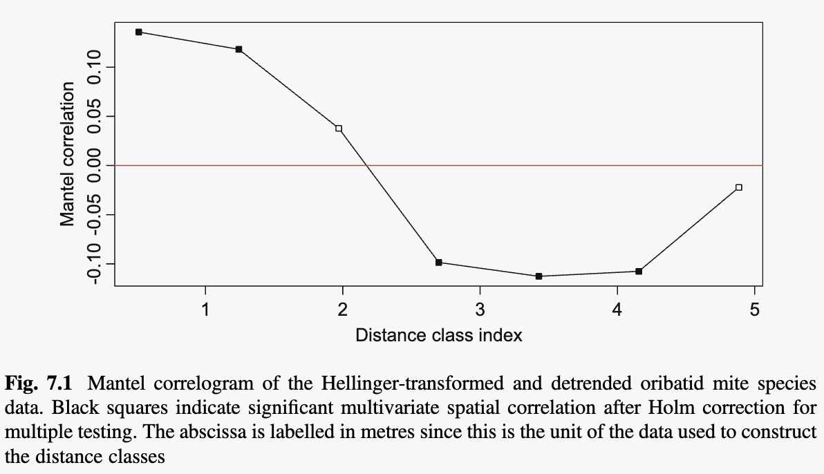
Fig. 7.1 as shown above, is a typical case that the correlation is positive for short distance, then descreases to negative values and levels out to a point that the correlation is non-significant.
spdep::sp.correlogram() takes one environmental variable and the geo distance matrix to test for univariate spatial correlation. See p.304 for details.
However for having both geographic distance and genetic distance in matrix, we need to pivot to the multivariate version of spatial correlogram, which is Mantel Correlogram Based on testing Mantel statistics \(r_M\), one is testing the correlation between two matrix subset based on geographical distance classes. A Multivariate Patial Mantel Correlogram is described and employed by Matesanz et al. (2011), which can filter out the effect of an environmental factor by providing a thrid matrix. This method requires however more careful evaluation.
Technically, mantel correlogram is computing a standardized \(r_M\) between a dissimilarity matrix among sites (samples) and a matrix where pairs of sites belonging to the same distance class receive value 0 and the other pairs, value 1. Which means if the genetic distances of sample pairs in one geo. distance class are lower than the others in other classes, then they will yield a higher \(r_M\) for that particular geo. distance class, stating that the sample within that geo. distance class is genetically similar than expected (using the rest of the sample as baseline or using the whole?), vice versa.