ASV <- read.delim(paste0(path, "data/ASV.txt"), sep = "\t", header = TRUE)
# ASV = abundance data of OTUs at sampling locations (OTU x location)
ENV <- read.delim(paste0(path, "data/ENV.txt"), sep = "\t", header = TRUE)
# ENV = environmental data of sampling locatoins
LOC <- read.delim(paste0(path, "data/Sample_Classification.tsv"), sep ="\t", header = T)
# LOC = Location data for sampling locations eg. depth / ocean layerDescriptive Community Ecology using NMDS
Multivariate Analysis
Mediterranean Micobiome
Abstract
This is the first post of the Mediterranean Microbial Network series.
- This is a meta-analysis for demonstration in M. Sc. Biology module Network Analysis in Ecology and Beyond offered by Prof. Dr. Jochen Fründ at University of Hamburg.
- The data used is credited to Deutschmann et al. (2024) and available in the original repo, as well as in our repo.
- Data wrangling was done by Jan Moritz Fehr.
Ocean Microbiome
We adopted the ocean microbial data processed and published by Deutschmann et al. (2024), and focused on the Mediterranean subset. Thank to the comprehensive record of ecological parameters, we were able to divide the dataset according to their depth. The data was originally categorized in 5 layers:
- Surface (SRF): 0 - 3 m
- Epipelagic (EPI): 12 - 50 m
- Deep-Chlorophyll Maximum (DCM): 40 - 130 m
- Mesopelagic (MES): 200 - 1000 m
- Bathypelagic (BAT): 1100 - 3300 m
We have combined EPI and DCM for the sake of simplicity and also because DCM is recognized as part of EPI. EPI is also called as sunlit zone, where solar resource could still be utilized by photosynthesis. As the red light being absorbed faster than the blue light, in MES, also known as twilight zone, there’s only dim blue light present, which can not be used for photosynthesis. The light will eventually disappear in BAT, at which depth the most area of Mediterranean Sea hits the sea floor.
In each layer, the species composition besides microorganism is different: in SRF and EPI, phytoplanktons are able to import solar energy into the ecosystem and this attracts small zooplanktons to feed at this depth. As photosynthesis becomes no longer possible in MES, it is home to many nektons: fishes, squids, planktonic crustaceans, etc. In BAT, as we approach the sea floor, benthic fauna becomes an important part. Such differences in interaction partners will also affect microorganism communities. But in what extent? Or how are the communities different? The co-occurrence / association data of the microorganism can help us answer those questions.
Deutschmann et al. (2024) published an Amplicon Sequences Variants (ASV) abundance data, which comprises an abundance matrix in the form that each row represents a sample site and each column represents an OTU (Operational Taxonomic Unit, commonly used in microbiology as proxies for species concept). This matrix directly represents an adjacency matrix for a species-location bipartite network.
For more information about ocean layers, kindly see Know Your Ocean from WHOI.
Lets get the data imported and start with some basic data wrangling:
MS is now a dataframe comprising n = 145 rows as sample sites and p = 3208 columns of OTU, which stores the abundance data in the form of an adjacency matrix. There are additional 16 columns at the end for ecological data.
Non-metric Multi-Dimensional Scaling (NMDS)
The most intuitive way to have an overview on the community is to plot them out, NMDS is the most common way to do this.
library(tidyverse)
library(vegan)

set.seed(1)

ab.mtx <- as.matrix(MS[, 1:ab.mtx.ncol]) # extract abundance matrix
Data Preparation
Taking a brief look at the data, it’s very clear that out microbial data is actually largely skewed. There are a few species with extremely high reads, and a vast majority being very low frequent, and almost 85% of the cells in our matrix are zero.
ab.mtx[ab.mtx == 0] %>% length() / ab.mtx %>% length()[1] 0.8453521max(ab.mtx)[1] 59282hist(ab.mtx)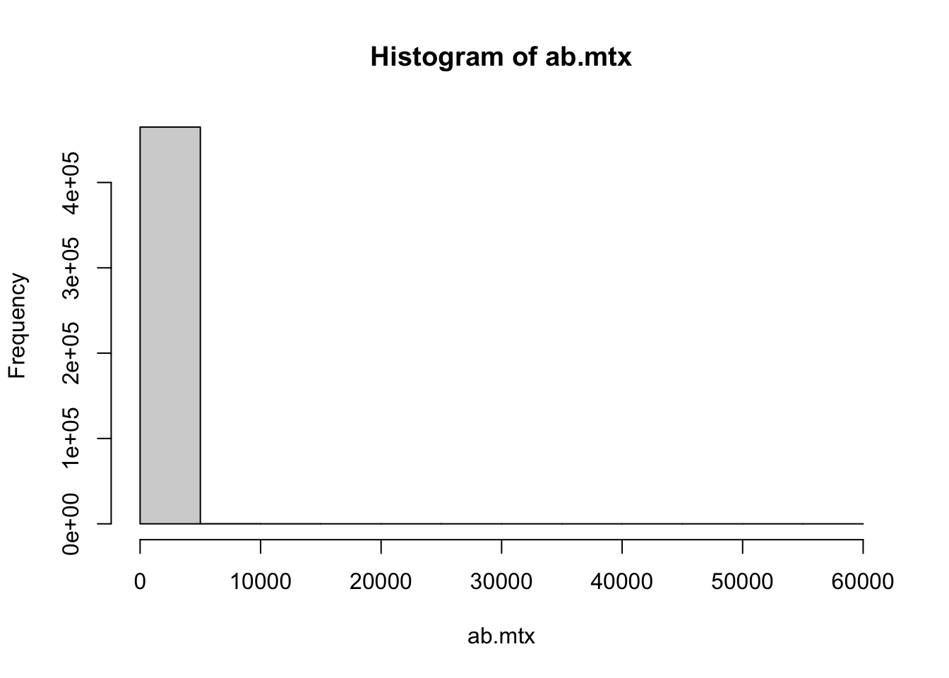
It’s worth noting that vegan::metaMDS(), the function that does the calculation for NMDS, will try to autotransform the data if not specified autotransform = False. In our case, considering the extreme skewness of the data and clear pattern, which transforming method to use did not really make big differences. But this is not always true. One should select these methods cautiously. Hellinger transformation is one way to reduce the weight of extremely high value.
ab.mtx.tf <- decostand(ab.mtx, "hellinger")
hist(ab.mtx.tf)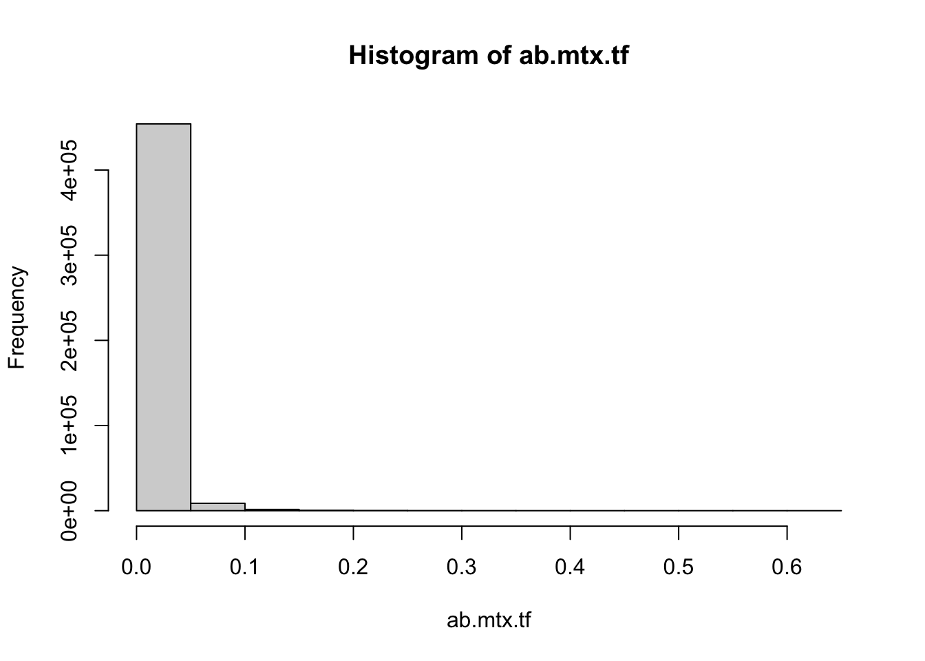
Perform NMDS
Every community ecologist should be familiar with the basic idea of NMDS, which is dimension reduction. It converts our n x p matrix into an n x n dissimilarity matrix. This steps allows flexible decision on how the distances should be calculated. A common choice while dealing with species composition is the Bray-Curtis dissimilarity, as its semi-metric approach takes both presence/absence and abundance information into account. It is also default to metaMDS().
NMDS differs a bit from other ordination methods, like PCA, in handling the distances and calculating axes and coordinates. Its non-metric nature decided that the distance on the final plot does not represents the distances between dataset, but the ranking order. It also therefore, does not try to maximize the variability in axes, which means the axes are completely arbitrary and this technique is mainly used for visualization only (Bakker 2024).
Before starting NMDS, we have to specify k, which gives the number of axes we want to have. NMDS will then take iterative process to adjust the scaling. After each iteration, it calculates a stress values showing how nice the ordination represents real data. The value ranges from 0 to 1, where 0 means a perfect fit. It however indicates danger for interpreting the ordination already from 0.2. Generally a stress value under 0.1 is considered a good result (Clarke 1993; Bakker 2024).
NMDS <- metaMDS(ab.mtx.tf, k=2, autotransform = F, trymax = 50)NMDS Plot using {ggplot2}
There are several plotting functions from {vegan}, but since we were trying to make a fancy poster, I brought out my old script to make fully controlled plot with {ggplot2}.
# Extract coordinates
siteCoord <- as_tibble(scores(NMDS)$sites)
spCoord <- as_tibble(scores(NMDS)$species)

# Import aesthetics setting
aes_setting <- function() {
    list(
        theme_minimal() +
        theme(
            aspect.ratio = 1,
            plot.title = element_text(size = 12, face = "bold", family = "Times New Roman", hjust = 0.5),
            axis.ticks.length = unit(-0.05, "in"),
            axis.text.y = element_text(margin=unit(c(0.3,0.3,0.3,0.3), "cm")),
            axis.text.x = element_text(margin=unit(c(0.3,0.3,0.3,0.3), "cm")),
            axis.ticks.x = element_blank(),
            plot.background = element_blank(),
            legend.background = element_blank(),
            panel.background = element_rect(color = NULL, fill = "white"),
            panel.border = element_rect(color = "black", fill = "transparent"),
            panel.grid = element_line(linewidth = 0.3)
        )
    )
}

# Plot the species
p.NMDS.sp <- ggplot() +
    geom_point(data = spCoord, aes(x = NMDS1, y = NMDS2), size = 2, shape = 3, color = "grey", alpha = 0.25) +
    aes_setting() +
    theme(aspect.ratio = 1) +
    coord_equal()

p.NMDS.sp
As simple as that, we have our species plotted. But we are not really interested in individual species, instead, the community at different sites. For that purpose, we have to first pass the environmental data of each site into siteCooord.
# Extract environmental data, combine DCM with EPI
env <- MS[, (ab.mtx.ncol+1):ncol(MS)] %>%
    mutate(layer = case_when(layer == "DCM" ~ "EPI", .default = layer))
siteCoord_env <- cbind(siteCoord, env)

# Order the layer
siteCoord_env_ordered <- siteCoord_env %>% mutate(layer = factor(layer, levels = c("SRF", "EPI", "MES", "BAT")))
Then we can plot them as usual:
# Define colors for the layers
depth.colors <- c(
"SRF" = "#6CCCD6",
"EPI" = "#007896",
"MES" = "#004359",
"BAT" = "#001C25"
)
depth.shapes <- c(
"SRF" = 15,
"EPI" = 16,
"MES" = 17,
"BAT" = 18
)
p.NMDS.st <- ggplot() +
geom_point(data = siteCoord_env_ordered, aes(x = NMDS1, y = NMDS2, color = layer, shape = layer), size = 3.5, alpha = 0.8) +
aes_setting() +
theme(aspect.ratio = 1) +
scale_color_manual(values = depth.colors) +
scale_shape_manual(values = depth.shapes) +
guides(color = guide_legend("Layer"), fill = "none", shape = guide_legend("Layer"))
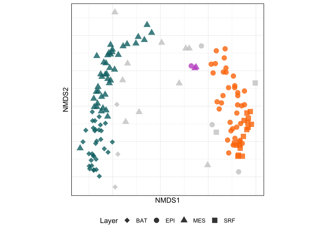
p.NMDS.st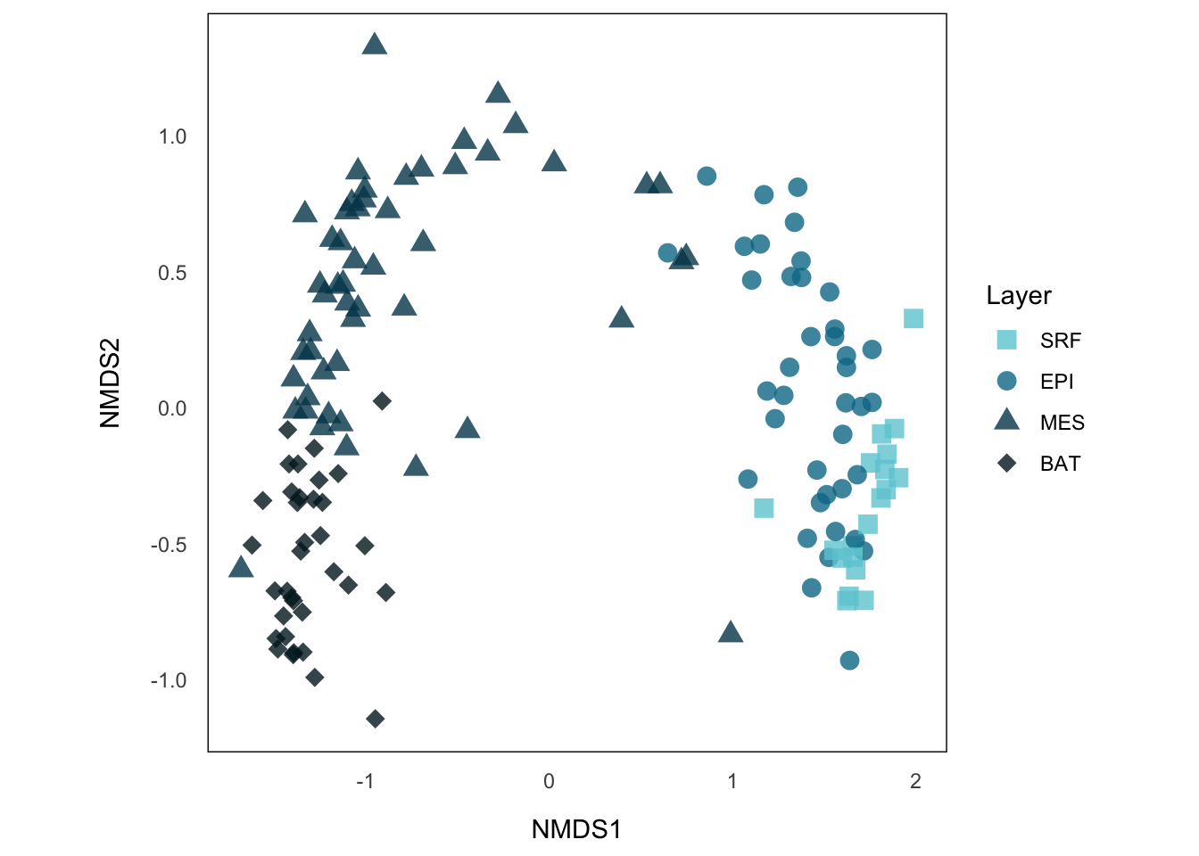
Now, this is telling us more information, we can see that sample sites from the same layer tend to cluster together, where MES and BAT form a big group distinct from EPI and SRF. A common way to show such categorical data in NMDS is to draw a convex hull on those clusters.
NMDS Hullplot using {ggplot2}
The basic idea is simply use chull() to identify the points from the same cluster that are on the border of the hull and draw a polygon using those points. But the problem is that we have some outliers here, especially from MES (those which neighboring BAT and SRF). These points will surely become the one defining the convex hull, and make the hull covering much more area than the cluster really does.
To address this, I additionally calculate the euclidean centroids of each cluster and filter out outliers by comparing their distances to the centroids with the median distances to the centroids from all points within the same cluster. Those points that has a distance larger than a threshold calculated from median distance with defined multiplier will not be included.
See the result if we do not exclude those points
# Calculate the coordinates of the hull border
outliner <- function(coord, group_var,  threshold_factor = 2, threshold_func = median) {
    centroid <- colMeans(coord[, c(1, 2)])
    centroids <- matrix(c(rep(centroid[1], nrow(coord)), rep(centroid[2], nrow(coord))), ncol = 2)

    # Euclidean distances
    coord$distances <- sqrt(rowSums((coord[, c(1, 2)] - centroids)^2))

    # Set threshold
    threshold <- threshold_factor * threshold_func(coord$distances)

    # filter out points with distance larger than threshold
    coord_in <- coord[coord$distances <= threshold, ]

    outline_indices <- chull(coord_in[, c(1, 2)])

    return(list(
        borders = coord_in[outline_indices, ],
        centroid = c(centroid, group = group_var[[1]])
    ))
}
threshold_factor controls how conservative or inclusive the convex hull should be drawn. Then we apply this process to each category and extract the hull border coordinatees for ggplot. threshold_func defines which function to use for choosing baseline of the threshold. Default is set to median() here since mean() can skew the baseline if any extreme outlier exists.
# Using ordered factor from `siteCoord_env_ordered` can't successfully pass the layer name through the pipeline
layer.siteCoord <- siteCoord_env %>%
group_by(layer) %>%
group_map(~ outliner(.x, .$layer), .keep = T) %>%
`names<-`(group_keys(siteCoord_env %>% group_by(layer))[[1]]) %>%
do.call(what = rbind, args = .) %>%
as.data.frame()
# Extract border and centroid coordinates
borders.pCoord <- layer.siteCoord[["borders"]] %>% bind_rows()
centroids.pCoord <- layer.siteCoord[["centroid"]] %>% bind_rows() %>% mutate(NMDS1 = as.numeric(NMDS1), NMDS2 = as.numeric(NMDS2))
p.NMDS.st.hull <- p.NMDS.st +
geom_polygon(data = borders.pCoord, aes(x = NMDS1, y = NMDS2, fill = layer), alpha = 0.5) + # hull
geom_text(data = centroids.pCoord, aes(x = NMDS1, y = NMDS2, label = group)) +
scale_fill_manual(values = depth.colors)
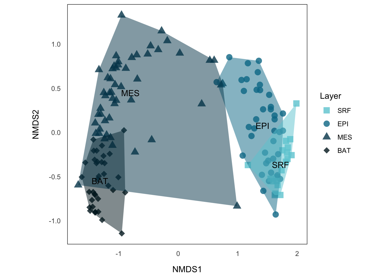
p.NMDS.st.hull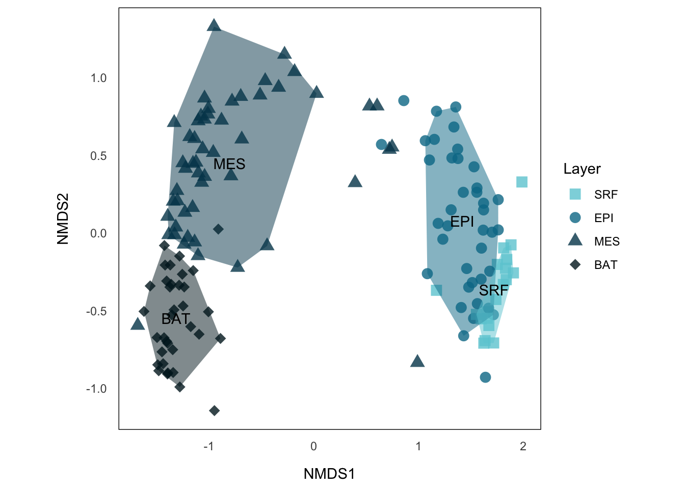
Now, each layer forms a cluster that does not have much overlap with others, except EPI and SRF, which also make sense, because even microorganism in SRF might have different interacting partners than the rest of EPI, the environmental condition and the general species compositions, in particular functionally, should be similar. This is also reflected by SRF on the right side of EPI with larger distance to MES or BAT.
The space between MES and EPI is not encapsulated by any of both, it reflects the “bridge” section, probably at which depth that both layers meet each other. There’s a numerical depth data in env, which is principally continuous data complementing our layer categories. While we use hull plot to visualize categeories in NMDS, we can use contour line to visualize continuous variables.
Fitting smooth surface
If we imagine the variables we want to display as the third dimension of our points on NMDS, visualizing the variables becomes simply visualizing a 3-D structure on our 2-D plot. One of the solution is to fit the surface on our plot using vegan::ordisurf().
The way to extract contour line from vegan::ordisurf() and the function extract.xyz() are credited to Christopher Chizinski’s post.
library(geomtextpath)
extract.xyz <- function(obj) {
    print(obj)
  xy <- expand.grid(x = obj$grid$x, y = obj$grid$y)
  xyz <- cbind(xy, c(obj$grid$z))
  names(xyz) <- c("x", "y", "z")
  return(xyz)
}

depth.surf <- ordisurf(NMDS, env$depth, permutation = 999, na.rm = T, plot = F)
depth.contour <- extract.xyz(obj = depth.surf)
Family: gaussian
Link function: identity

Formula:
y ~ s(x1, x2, k = 10, bs = "tp", fx = FALSE)

Estimated degrees of freedom:
7.84  total = 8.84

REML score: 1057.237
p.NMDS.st.hull.cont <- p.NMDS.st.hull +
geom_textcontour(data = depth.contour, aes(x, y, z = z), color = "#c4438c")
p.NMDS.st.hull.cont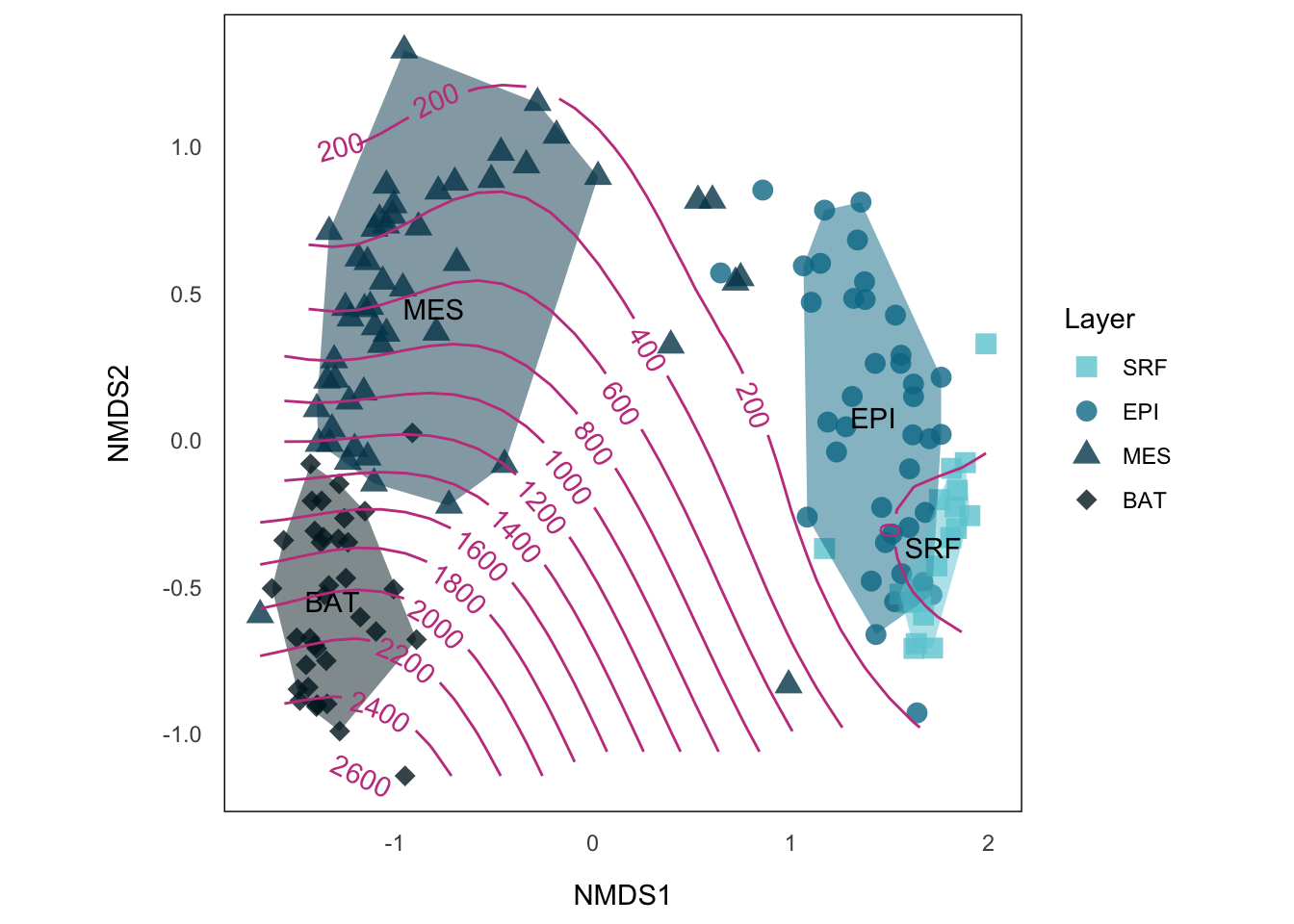
We see those points on the MES/EPI border could be perfectly explained by the depth.
Detecting Density-based Cluster with {dbscan}
Another interesting way to analyse the community structure more objectively is to cluster the points purely based on their location on NMDS, without taking the environmental parameters into account. Now speaking of cluster, you might be thinking about drawing another convex shape, probably an oval or a circle around the data points. This is however not applicable in our case, and usually in many real-life cases: out data points in the NMDS space clearly from clusters whose shapes are irregular. To address this issue, we use a density-based clustering algorithm called DBSCAN. The main idea of a density-based cluster is that the shape of the cluster is arbitrary, and it is defined by a continuous space with high density of data points, which suggests they are similar to each other, and clusters are separated by low-density region in between. This method can effectively filter out the outliners and noises, in a more robust way than just setting threshold on the distance to the centroid. And also, while the clusters are now in arbitrary shapes, the centroids become meaningless too.
The main idea of detecting high density area is to categorize data points by the distance to their neighbors into core points and border points. Contiguous connection (neighboring) of core points represents the contiguous dense area, where border points identify the periphere. All interconnected core points and border points are the same cluster, points that are not connected to any core point are noises. You can find more details about the algorithm and the package in their vignettes and a nice graphic introduction by StatQuest.
library(dbscan)

?dbscan()
We need to specify two parameters for DBSCAN, which affect how we identify the core points: the minimum points (including the point itself) required in a point’s epsilon neighborhood for becoming a core point (minPts) and the size of the epsilon neighborhood (eps). Bigger the minPts the more difficult for a point to become a core point, a rule of thumb is to choose the number of axis we have + 1, which will be 3 in our case. Choice of eps value, however, depends on how scattered the points are. The bigger the eps, the easier for a point to reach the requirement we set with minPts to become a core point, and vice versa. To find an eps value that is not too high or too low, we can have a peak into how the distances between points look like:
kNNdistplot(siteCoord_env_ordered[,1:2], k = 2)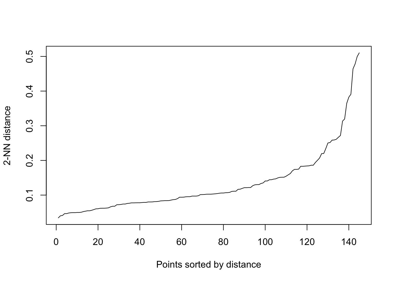
The plot shows every point’s distance to their k-th nearest neighbor (kNN), ordered ascending. The reason we are looking at the distances to their kNNs (2nd in our case) is because our minPts will be k + 1, so the distances shown are the maximum distances the points’ epsilon neighborhoods need to cover for becoming core points. What we want to identify is the knee of the curve, which is around y = 0.2, and it will be our eps value. Set the eps lower, we will lose a lot potential core points and prevent the nearby high dense areas connect with each other to form bigger cluster, this can be useful when we want to distinguish clusters stricter; if we set the eps at higher value, we will identify too much core points that eventually connect all clusters together as one.
kNNdistplot(siteCoord_env_ordered[,1:2], k = 2)
abline(h = 0.2, col = "red")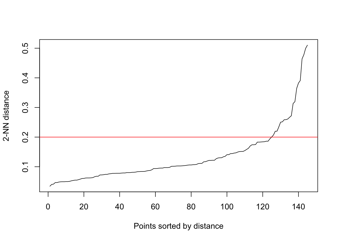
With parameters set, we simply
siteCoord_scan <- dbscan(siteCoord_env_ordered[,1:2], eps = 0.2, minPts = 3)

siteCoord_scan
DBSCAN clustering for 145 objects.
Parameters: eps = 0.2, minPts = 3
Using euclidean distances and borderpoints = TRUE
The clustering contains 3 cluster(s) and 18 noise points.
0 1 2 3
18 72 52 3
Available fields: cluster, eps, minPts, metric, borderPointssiteCoord_env_scan <- siteCoord_env %>% mutate(dbcluster = factor(siteCoord_scan$cluster))
ggplot() +
geom_point(data = siteCoord_env_scan, aes(x = NMDS1, y = NMDS2, color = dbcluster, shape = layer), size = 3.5, alpha = 0.8) +
scale_color_manual(values = c("#CCC", paletteer::paletteer_d("ltc::trio1")) %>% `names<-`(c(0:3))) +
scale_shape_manual(values = depth.shapes) +
aes_setting() +
labs(shape = "Layer") +
guides(color = "none") +
theme(
axis.text.x = element_blank(),
axis.text.y = element_blank(),
legend.position = "bottom",
legend.direction = "horizontal",
legend.box = "vertical"
)
But, what we did so far was basic descriptive work in community ecology. We still want to take a look into each community structure using network analysis. I will cover this in the next upcoming post. To be continued.
Reference
Bakker, Jonathan D. 2024. Applied Multivariate Statistics in R. University of Washington. https://uw.pressbooks.pub/appliedmultivariatestatistics/.
Clarke, K. R. 1993. “Non-Parametric Multivariate Analyses of Changes in Community Structure.” Australian Journal of Ecology 18 (1): 117–43. https://doi.org/10.1111/j.1442-9993.1993.tb00438.x.
Deutschmann, Ina M., Erwan Delage, Caterina R. Giner, Marta Sebastián, Julie Poulain, Javier Arístegui, Carlos M. Duarte, et al. 2024. “Disentangling Microbial Networks Across Pelagic Zones in the Tropical and Subtropical Global Ocean.” Nature Communications 15 (1): 126. https://doi.org/10.1038/s41467-023-44550-y.
Citation
BibTeX citation:
@online{hu2025,
  author = {Hu, Zhehao},
  title = {Descriptive {Community} {Ecology} Using {NMDS}},
  date = {2025-07-25},
  url = {https://zzzhehao.github.io/biology-research/community-ecology/MediMicro-NMDS.html},
  langid = {en},
  abstract = {This is the first post of the Mediterranean Microbial
    Network series.}
}
For attribution, please cite this work as:
Hu, Zhehao. 2025. “Descriptive Community Ecology Using
NMDS.” July 25, 2025. https://zzzhehao.github.io/biology-research/community-ecology/MediMicro-NMDS.html.
