# use install.packages() if not already installed.
library(tidyverse)
library(vegan)
library(Rtsne)
library(paletteer)
library(cli)

path <- "proteomics"Simple guide on performing TSNE
Multivariate Analysis
Abstract
Simpel guide on performing TSNE
Env setup
Data preparation
Data import:
- peak matrix should be the binned, but untransformed peak matrix. If already hellinger transformed, then just skip the
decostandstep later.
peakMatrix <- readRDS(file.path(path, "assets/tsne-1/peakmatrix_pc.rds"))
metadataSample <- readRDS(file.path(path, "assets/tsne-1/sample_metadata.rds"))
Hellinger transform
peakMatrix.hellinger <- decostand(peakMatrix, "hellinger")Important is that the row names of the peak matrix should correspond to a key column in metadata (reference table) so that each row in peak matrix can match to their metadata later. Here I have the column sampleName in meatadata dataframe and I check the rownames agains it:
str(metadataSample) # structure of the reference table'data.frame': 93 obs. of 10 variables:
$ sampleName : chr "VPSM001_1" "VPSM002_1" "VPSM003_1" "VPSM003_2" ...
$ name : chr "VPSM001_1.A1" "VPSM002_1.B1" "VPSM003_1.C1" "VPSM003_2.B9" ...
$ ID.maldi : chr "VPSM001" "VPSM002" "VPSM003" "VPSM003" ...
$ ID.DZMB2HH : chr "3641" "3808" "3823" "3823" ...
$ station : chr "61" "81" "81" "81" ...
$ gensp_morpho_ZH: chr "Haploniscus unicornis complex" "Haploniscus unicornis complex" "Haploniscus charcoti" "Haploniscus charcoti" ...
$ sex_ZH : chr "female" "female" NA NA ...
$ stage_ZH : chr NA NA NA NA ...
$ voucher_valid : chr "VPS001" "VPS002" "VPS003" "VPS003" ...
$ label : chr "VPSM001_1.A1_Haploniscus_unicornis_complex_female_3641_84" "VPSM002_1.B1_Haploniscus_unicornis_complex_female_3808_54" "VPSM003_1.C1_Haploniscus_charcoti_NA_3823_55" "VPSM003_2.B9_Haploniscus_charcoti_NA_3823_63" ...# extract rownames from the matrix
sampleName <- rownames(peakMatrix.hellinger)
head(sampleName)[1] "VPSM001_1" "VPSM002_1" "VPSM003_1" "VPSM003_2" "VPSM004_1" "VPSM005_1"# check all rownames has a match in the column of the dataframe
all(sampleName %in% metadataSample$sampleName) [1] TRUEDefine TSNE
We define a function that performs TSNE and plots it out, so the process can be scaled up later:
tsne <- function(
    perplexity,
    matrix,
    metadata,
    key_col,
    color_by,
    dims = 2,
    max_iter = 5000,
    seed = NULL
) {
    if (!is.null(seed)) {set.seed(seed)}

    tsne.res <- Rtsne(dims = dims, X = matrix, theta = 0.0, max_iter = max_iter, perplexity = perplexity)

    # extract tsne coordinates
    colnames(tsne.res$Y) <- LETTERS[c(24:26, 1:23)][1:ncol(tsne.res$Y)]
    tsne.coords <- as_tibble(tsne.res$Y)

    # glue tsne result with metadata
    tsne.matrix <- tsne.coords %>%
        bind_cols(tibble(!!key_col := sampleName)) %>%
        left_join(., metadata, by = key_col)

    # exit if not 2-dim TSNE
    if (dims != 2) {
        cli::cli_alert_danger("Plot option is only for 2-dimensional TSNE. Returning matrix only.")
        return(list(matrix = tsne.matrix, plot = NULL))
    }

    # Plot tsne
    tsne.plot <- ggplot() +
        geom_point(
            data = tsne.matrix,
            aes(
                x = X,
                y = Y,
                color = .data[[color_by]]),
            size = 3) +
        labs(title = paste0("t-SNE, perplexity = ", perplexity), x = "TSNE 1", y = "TSNE 2")  +
        theme_minimal() +
        theme(
            aspect.ratio = 1,
            plot.title = element_text(size = 12, face = "bold", family = "Times New Roman", hjust = 0.5),
            axis.ticks.length = unit(-0.05, "in"),
            axis.ticks = element_blank(),
            plot.background = element_blank(),
            legend.background = element_blank(),
            panel.background = element_rect(color = NULL, fill = "white"),
            panel.border = element_rect(color = "black", fill = "transparent"),
            panel.grid = element_line(linewidth = 0.3),
            legend.text = element_markdown()
        )

    return(list(matrix = tsne.matrix, plot = tsne.plot))
}
This function takes arguments:
- perplexity: numeric. Hyperparameter of TSNE. Should not be bigger than
3 * perplexity < nrow(matrix) - 1. Also see?Rtsne::Rtsne. - matrix: matrix. Peak matrix.
- metadata: data frame or tibble. Reference table, must contain one column against which the rownames of the matrix can be matched.
- key_col: character. Column name of the
metadatatable against which the rowname of the matrix should be matched. - color_by: character. Column name of the
metadatatable by which the dots in TSNE should be colored. - dims: numeric. Dimension of the TSNE. Default to 2. If greater than 2, only TSNE result matrix will be returned. If performing 3-dimensional TSNE,
{plotly}can visualize 3-dimensional data. - max_iter: numeric. Maximum iteration. Default to 5000.
- seed: numeric. Seed for reproducibility. Default to NULL.
and returns a list:
[[matrix]]: TSNE result.- `[[plot]]``: TSNE visualization with ggplot (2-dim TSNE only).
Perform TSNE
As you see, there’s a hyperparameter perplexity for TSNE, whose optimal value could not be determined beforehand. There’s an empirical rule for the range to be consider, but the best value varies from dataset to dataset. Based on the suggestion from {Rtsne} package, we calculate the upper limit for this dataset:
perplexity.max <- floor((nrow(peakMatrix)-1)/3)
perplexity.max
[1] 28Then we try a series of TSNE with different perplexity starting from 5 to 28 by every 5, that means c(5, 10, 15, 20, 25), or in a more programmatical way:
perplexity.step <- 5
perplexity <- perplexity.step*seq(perplexity.max%/%perplexity.step)
Then we perform TSNE for each perplexity:
tsne.list <- map(
    perplexity,
    ~tsne( # purrr-style anonymous function
        perplexity = .x,
        matrix = peakMatrix,
        metadata = metadataSample,
        key_col = "sampleName",
        color_by = "gensp_morpho_ZH",
        seed = 1
    )
)

map(tsne.list, ~.x[["plot"]]) %>% walk(~print(.x))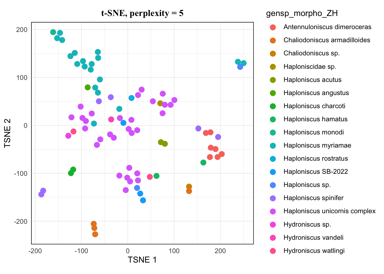
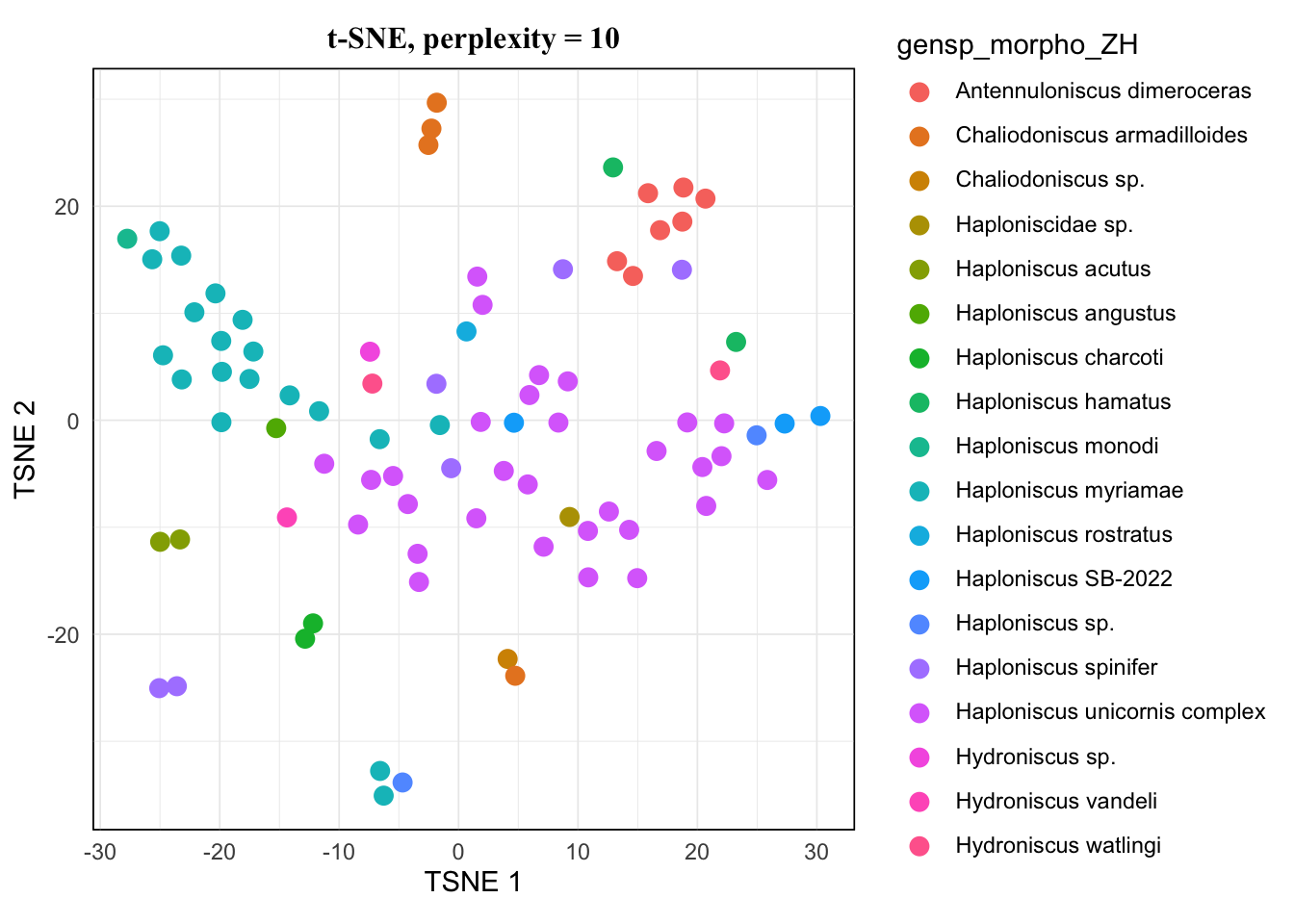
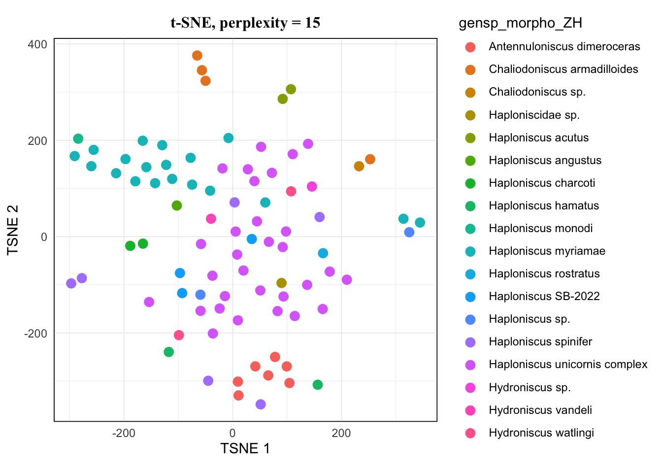
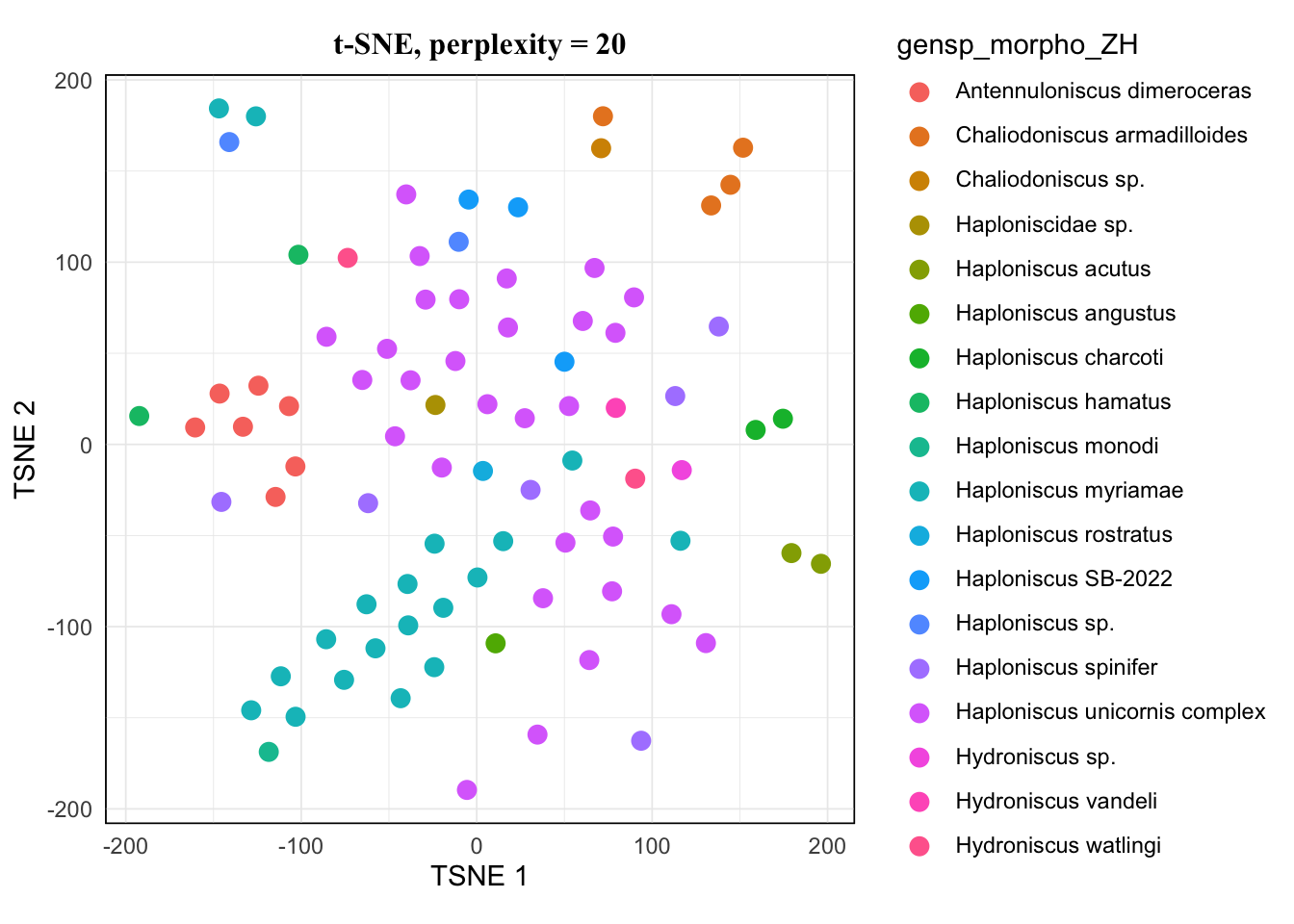

The pattern of 20 and 25 looked the same, and 15 hardly showed difference from them either. I would avoid 5 as it’s very low, so for a balanced result, I would take 10 for this dataset.
For more about how TSNE behaves and what perplexity means for it, see this article.
Visualization
Now we pick the plot and do some adjustment for publication:
tsne.res <- tsne(
    perplexity = 10,
    matrix = peakMatrix,
    metadata = metadataSample,
    key_col = "sampleName",
    color_by = "gensp_morpho_ZH",
    seed = 1
)
tsne.plot <- tsne.res[["plot"]]
If you print out tsne.plot at this step, notice that plot is identical to the one we saw earlier, as we have set the seed to the same value and therefore locked the random process. If we didn’t do so, the clustering result would be slightly different and therefore also the placement of the dots.
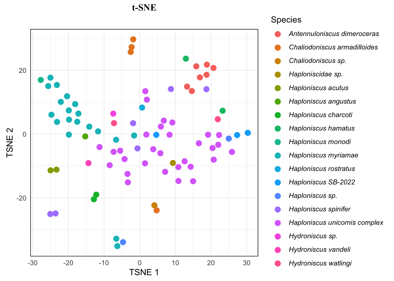
Then we can make adjustment for the plot, here’s just an example, more details see:
tsne.plot <- tsne.plot +
    labs(
        title = "t-SNE",
        subtitle = "",
        color = "Species"
    )

tsne.plot
You can also look for the best color palette for your dataset here and change the color palette by adding scale_color function family from {ggplot2} and {paletteer}.
tsne.plot <- tsne.plot +
    scale_color_paletteer_d("ggthemes::Miller_Stone")
Exporting the plot can be done by ggsave(), adjust parameter as needed.
ggsave("tsne_plot.svg", tsne.plot, width = 10, height = 8)It’s possible to make the species name in legend italic (require package {ggtext}), but the formatting step needs to be done before TSNE:
library(ggtext)

# format species name in reference table
metadataSample.format <- metadataSample %>%
    mutate(gensp_morpho_ZH = sprintf("*%s*", gensp_morpho_ZH))

# perform tsne
tsne.res <- tsne(10, peakMatrix, metadataSample.format, "sampleName", "gensp_morpho_ZH", seed = 1)

# extract tsne plot
tsne.plot <- tsne.res[["plot"]]

# format tsne plot
tsne.plot +
    labs(
        title = "t-SNE",
        subtitle = "",
        color = "Species"
    ) +
    theme(
        legend.text = element_markdown() # treat legend text as markdown text
    )
As you see, this just wraps the species name in the reference table inside single *, which is standard markdown syntax for italic, and we let ggplot treat the text in legend as markdown text. So it’s also possible to exclude open nomenclature (such as “sp.”, “cf.”, etc) from italicizing, but it requires a whole bunch of functions for taxa name matching, etc. So it’s not included here.
Reference
Citation
BibTeX citation:
@online{hu2026,
  author = {Hu, Zhehao},
  title = {Simple Guide on Performing {TSNE}},
  date = {2026-03-27},
  url = {https://zzzhehao.github.io/post/research/techs/proteomics_tsne.html},
  langid = {en},
  abstract = {Simpel guide on performing TSNE}
}
For attribution, please cite this work as:
Hu, Zhehao. 2026. “Simple Guide on Performing TSNE.” March
27, 2026. https://zzzhehao.github.io/post/research/techs/proteomics_tsne.html.
